Hands-on Introduction to Torch
Ronan Collobert
original version by Soumith Chintala
Get started
Get this itorch notebook
Run itorch
itorch notebookGoal of this talk
- Understand torch and the neural networks package at a high-level.
- Train a small neural network on CPU and GPU
What is Torch?
Torch is an scientific computing framework based on Lua[JIT] with strong CPU and CUDA backends.
Strong points of Torch:
- Efficient Tensor library (like NumPy) with an efficient CUDA backend
- Neural Networks package -- build arbitrary acyclic computation graphs with automatic differentiation
- also with fast CUDA and CPU backends
- Good community and industry support - several hundred community-built and maintained packages.
- Easy to use Multi-GPU support and parallelizing neural networks
http://torch.ch
https://github.com/torch/torch7/wiki/Cheatsheet
Before getting started
- Based on Lua and C.
- Currently runs on LuaJIT (Just-in-time compiler) which is fast and supports FFI.
- Lua is pretty close to javascript.
- variables are global by default, unless
localkeyword is used - Only has one data structure built-in, a table:
{}. Doubles as a hash-table and an array. - 1-based indexing.
foo:bar()is the same asfoo.bar(foo)- Lua glues C/C++ libraries together
Develop fast (scripting language), run fast (minor overhead, C backend)
- The basic brick is the Tensor object
- n-dimensional array
used to store any kind of data
The torch package provides tensors... hundred of packages are built upon it.
Getting Started
Lua Types
Lua has 8 main types:
print(type(nil))
print(type(true))
print(type(10.4*3))
print(type("Hello world"))
print(type(function() print("Hello world") end))
print(type({a=3, b=4}))
print(type(torch.Tensor()))
The thread type will not be covered by this tutorial. Note that userdata allows to create C objects (like several Torch objects), and define your own type system over them.
Strings, numbers, tables - a tiny introduction
a = 'hello'
print(a)
b = {}
b[1] = a
print(b)
b[2] = 30
for i=1,#b do -- the # operator is the length operator in Lua
    print(b[i])
end
Tensors
a = torch.Tensor(5,3) -- construct a 5x3 matrix, uninitialized
a = torch.rand(5,3)
print(a)
Views
A tensor is a view over a piece of memory (a storage)
print(a:storage())
Torch relies heavily on views: - narrow(dim, idx, size) - select(dim, idx) - unfold(dim, kw, dw) - view(dim1, dim2, dim3, ...) - index operator [{}]
print(a:narrow(1, 3, 2))
Remember that view = pointer in a storage
an = a:narrow(1, 3, 2)
an:zero()
print(a)
a:select(2, 2):fill(3.14)
print(a)
print(a:size())
print(a:stride())
print(a:storageOffset())
print(a:select(2, 2):size())
print(a:select(2, 2):stride())
print(a:select(2, 2):storageOffset())
Math operations
See torch documentation for a survey on available math operations.
b=torch.rand(3,4)
-- matrix-matrix multiplication: syntax 1
a*b
-- matrix-matrix multiplication: syntax 2
torch.mm(a,b)
-- matrix-matrix multiplication: syntax 3
c=torch.Tensor(5,4)
c:mm(a,b) -- store the result of a*b in c
CUDA Tensors
Tensors can be moved onto GPU using the :cuda function
require 'cutorch';
a = a:cuda()
b = b:cuda()
c = c:cuda()
c:mm(a,b) -- done on GPU
Functions
N = 5

-- make sure everybody has the same random seed
torch.manualSeed(1234)

-- create a random NxN matrix
A = torch.rand(N, N)

-- make it symmetric positive
A = A*A:t()

-- make it definite
A:add(0.001, torch.eye(N))

-- add a linear term
b = torch.rand(N)

-- create a quadratic form
function J(x)
    return 0.5*x:dot(A*x)-b:dot(x)
end
Function call, here at a random point
print(J(torch.rand(N)))
Exercise: find the minimum of the quadratic function
We can inverse the matrix
xs = torch.inverse(A)*b
print(string.format('J(x^*) = %g', J(xs)))
Or we can do a gradient descent!
function dJ(x)
  return A*x-b
end
We define some current solution:
x = torch.rand(N)
and then apply gradient descent (with a given learning rate lr) for a while:
lr = 0.01
for i=1,20000 do
  x = x - dJ(x)*lr
  -- we print the value of the objective function every 1000 iterations
  if i % 1000 == 0 then
    print(string.format('at iter %d J(x) = %f', i, J(x)))
  end
end
Neural Networks
Neural networks in Torch can be constructed using the nn package.
require 'nn';
Modules are the bricks used to build neural networks. Each are themselves neural networks, but can be combined with other networks using containers to create complex neural networks
For example, look at this network that classfies digit images: 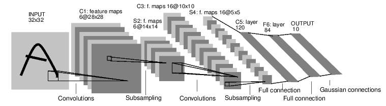
It is a simple feed-forward network.
It takes the input, feeds it through several layers one after the other, and then finally gives the output.
Such a network container is nn.Sequential which feeds the input through several layers.
net = nn.Sequential()

-- 1 input image channel, 6 output channels, 5x5 convolution kernel
net:add(nn.SpatialConvolution(1, 6, 5, 5))

-- A max-pooling operation that looks at 2x2 windows and finds the max.
net:add(nn.SpatialMaxPooling(2,2,2,2))

-- non-linearity
net:add(nn.Tanh())

-- additional layers
net:add(nn.SpatialConvolution(6, 16, 5, 5))
net:add(nn.SpatialMaxPooling(2,2,2,2))
net:add(nn.Tanh())

-- reshapes from a 3D tensor of 16x5x5 into 1D tensor of 16*5*5
net:add(nn.View(16*5*5))

-- fully connected layers (matrix multiplication between input and weights)
net:add(nn.Linear(16*5*5, 120))
net:add(nn.Tanh())
net:add(nn.Linear(120, 84))
net:add(nn.Tanh())

-- 10 is the number of outputs of the network (10 classes)
net:add(nn.Linear(84, 10))
print('Lenet5\n', tostring(net));
Other examples of nn containers are shown in the figure below: 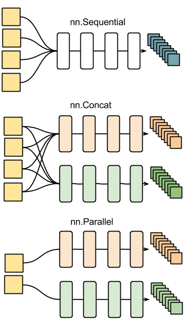
Every neural network module in torch has automatic differentiation. It has a :forward(input) function that computes the output for a given input, flowing the input through the network. and it has a :backward(input, gradient) function that will differentiate each neuron in the network w.r.t. the gradient that is passed in. This is done via the chain rule.
input = torch.rand(1,32,32) -- pass a random tensor as input to the network
output = net:forward(input)
print(output)
net:zeroGradParameters() -- zero the internal gradient buffers of the network (will come to this later)
gradInput = net:backward(input, torch.rand(10))
print(#gradInput)
One can then update the parameters with
net:updateParameters(0.001) -- provide a learning rate
Criterion: Defining a loss function
When you want a model to learn to do something, you give it feedback on how well it is doing. This function that computes an objective measure of the model's performance is called a loss function.
A typical loss function takes in the model's output and the groundtruth and computes a value that quantifies the model's performance.
The model then corrects itself to have a smaller loss.
In Torch, loss functions are implemented just like neural network modules, and have automatic differentiation.
They have two functions - forward(input, target) - backward(input, target)
For example:
-- a negative log-likelihood criterion for multi-class classification
criterion = nn.CrossEntropyCriterion()

-- let's say the groundtruth was class number: 3
criterion:forward(output, 3)
gradients = criterion:backward(output, 3)
gradInput = net:backward(input, gradients)
Review of what you learnt so far
- Network can have many layers of computation
- Network takes an input and produces an output in the
:forwardpass - Criterion computes the loss of the network, and it's gradients w.r.t. the output of the network.
- Network takes an (input, gradients) pair in it's
:backwardpass and calculates the gradients w.r.t. each layer (and neuron) in the network.
Missing details
A neural network layer can have learnable parameters or not.
A convolution layer learns it's convolution kernels to adapt to the input data and the problem being solved.
A max-pooling layer has no learnable parameters. It only finds the max of local windows.
A layer in torch which has learnable weights, will typically have fields .weight (and optionally, .bias)
m = nn.SpatialConvolution(1,3,2,2) -- learn 3 2x2 kernels
print(m.weight) -- initially, the weights are randomly initialized
print(m.bias) -- The operation in a convolution layer is: output = convolution(input,weight) + bias
There are also two other important fields in a learnable layer. The gradWeight and gradBias. The gradWeight accumulates the gradients w.r.t. each weight in the layer, and the gradBias, w.r.t. each bias in the layer.
Training the network
For the network to adjust itself, it typically does this operation (if you do Stochastic Gradient Descent):
weight = weight - learningRate * gradWeight [equation 1]
This update over time will adjust the network weights such that the output loss is decreasing.
Okay, now it is time to discuss one missing piece. Who visits each layer in your neural network and updates the weight according to Equation 1? - You can do your own training loop - Pro: easy customization for complicated network - Con: code duplication
- You can use existing packages
- optim
- nn.StochasticGradient
We shall use the simple SGD trainer shipped with the neural network module: nn.StochasticGradient.
It has a function :train(dataset) that takes a given dataset and simply trains your network by showing different samples from your dataset to the network.
What about data?
Generally, when you have to deal with image, text, audio or video data, you can use standard functions like: image.load or audio.load to load your data into a torch.Tensor or a Lua table, as convenient.
Let us now use some simple data to train our network.
We shall use the CIFAR-10 dataset, which has the classes: 'airplane', 'automobile', 'bird', 'cat', 'deer', 'dog', 'frog', 'horse', 'ship', 'truck'.
The images in CIFAR-10 are of size 3x32x32, i.e. 3-channel color images of 32x32 pixels in size. 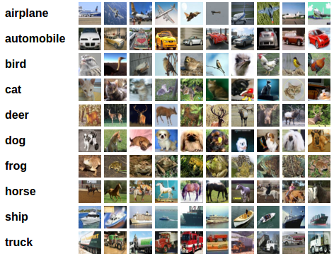
The dataset has 50,000 training images and 10,000 test images in total.
We now have 5 steps left to do in training our first torch neural network 1. Load and normalize data 2. Define a Neural Network 3. Define Loss function 4. Train network on training data 5. Test network on test data.
1. Load and normalize data
Today, in the interest of time, we prepared the data before-hand into a 4D torch ByteTensor of size 10000x3x32x32 (training) and 10000x3x32x32 (testing) Let us download the data...
os.execute('wget -c https://s3.amazonaws.com/torch7/data/cifar10torchsmall.zip')
os.execute('unzip -o cifar10torchsmall.zip')
And let's inspect it!
trainset = torch.load('cifar10-train.t7')
testset = torch.load('cifar10-test.t7')
classes = {'airplane', 'automobile', 'bird', 'cat',
           'deer', 'dog', 'frog', 'horse', 'ship', 'truck'}
print(trainset)
print(#trainset.data)
For fun, let us display an image:
itorch.image(trainset.data[100]) -- display the 100-th image in dataset
print(classes[trainset.label[100]])
Now, to prepare the dataset to be used with nn.StochasticGradient, a couple of things have to be done according to it's documentation. 1. The dataset has to have a :size() function. 2. The dataset has to have a [i] index operator, so that dataset[i] returns the ith sample in the datset.
Both can be done quickly:
-- ignore setmetatable() for now, it is a feature beyond the scope of this tutorial.
-- It sets the index operator.

setmetatable(trainset,
    {__index = function(t, i)
                    return {
                        t.data[i],
                        t.label[i]
                    }
                end}
);

function trainset:size()
    return self.data:size(1)
end

-- converts the data from a ByteTensor to a DoubleTensor.
trainset.data = trainset.data:double()
print(trainset:size()) -- just to test
print(trainset[33]) -- load sample number 33.
itorch.image(trainset[33][1])
One of the most important things you can do in conditioning your data (in general in data-science or machine learning) is to make your data to have a mean of 0.0 and standard-deviation of 1.0.
Let us do that as a final step of our data processing.
We are going to do a per-channel normalization
-- remember: our dataset is #samples x #channels x #height x #width
-- this picks {all images, 1st channel, all vertical pixels, all horizontal pixels}
redChannel = trainset.data:select(2, 1)
print(#redChannel)
Moving back to mean-subtraction and standard-deviation based scaling, doing this operation is simple, using the indexing operator that we learnt above:
mean = {} -- store the mean, to normalize the test set in the future
stdv  = {} -- store the standard-deviation for the future
for i=1,3 do -- over each image channel
    mean[i] = trainset.data:select(2, 1):mean() -- mean estimation
    print('Channel ' .. i .. ', Mean: ' .. mean[i])
    trainset.data:select(2, 1):add(-mean[i]) -- mean subtraction

    stdv[i] = trainset.data:select(2, i):std() -- std estimation
    print('Channel ' .. i .. ', Standard Deviation: ' .. stdv[i])
    trainset.data:select(2, i):div(stdv[i]) -- std scaling
end
Our training data is now normalized and ready to be used.
2. Time to define our neural network
We use here a LeNet-like network, with 3 input channels and threshold units (ReLU):
net = nn.Sequential()
net:add(nn.SpatialConvolution(3, 6, 5, 5))
net:add(nn.SpatialMaxPooling(2,2,2,2))
net:add(nn.Threshold())

net:add(nn.SpatialConvolution(6, 16, 5, 5))
net:add(nn.SpatialMaxPooling(2,2,2,2))
net:add(nn.Threshold())

net:add(nn.View(16*5*5))

net:add(nn.Linear(16*5*5, 120))
net:add(nn.Threshold())
net:add(nn.Linear(120, 84))
net:add(nn.Threshold())
net:add(nn.Linear(84, 10))
3. Let us define the Loss function
Let us use the cross-entropy classification loss. It is well suited for most classification problems.
criterion = nn.CrossEntropyCriterion()
4. Train the neural network
This is when things start to get interesting.
Let us first define an nn.StochasticGradient object. Then we will give our dataset to this object's :train function, and that will get the ball rolling.
trainer = nn.StochasticGradient(net, criterion)
trainer.learningRate = 0.001
trainer.maxIteration = 5 -- just do 5 epochs of training.
trainer:train(trainset)
5. Test the network, print accuracy
We have trained the network for 5 passes over the training dataset.
But we need to check if the network has learnt anything at all.
We will check this by predicting the class label that the neural network outputs, and checking it against the ground-truth. If the prediction is correct, we add the sample to the list of correct predictions.
Okay, first step. Let us display an image from the test set to get familiar.
print(classes[testset.label[100]])
itorch.image(testset.data[100])
Now that we are done with that, let us normalize the test data with the mean and standard-deviation from the training data.
testset.data = testset.data:double()   -- convert from Byte tensor to Double tensor
for i=1,3 do -- over each image channel
    local channel = testset.data:select(2, i)
    channel:add(-mean[i]) -- mean subtraction
    channel:div(stdv[i]) -- std scaling
    print(string.format('channel %d: mean = %f stdv = %f', i, channel:mean(), channel:std()))
end
-- for fun, print the mean and standard-deviation of example-100
horse = testset.data[100]
print(horse:mean(), horse:std())
Okay, now let us see what the neural network thinks these examples above are:
print(classes[testset.label[100]])
itorch.image(testset.data[100])
predicted = net:forward(testset.data[100])
-- show scores
print(predicted)
You can see the network predictions. The network assigned a probability to each classes, given the image.
To make it clearer, let us tag each probability with it's class-name:
for i=1,predicted:size(1) do
    print(classes[i], predicted[i])
end
Alright, fine. How many in total seem to be correct over the test set?
correct = 0
for i=1,10000 do
    local groundtruth = testset.label[i]
    local prediction = net:forward(testset.data[i])
    local confidences, indices = torch.sort(prediction, true)  -- true means sort in descending order
    if groundtruth == indices[1] then
        correct = correct + 1
    end
end
print(correct, 100*correct/10000 .. ' % ')
That looks waaay better than chance, which is 10% accuracy (randomly picking a class out of 10 classes). Seems like the network learnt something.
Hmmm, what are the classes that performed well, and the classes that did not perform well:
class_performance = {0, 0, 0, 0, 0, 0, 0, 0, 0, 0}
for i=1,10000 do
    local groundtruth = testset.label[i]
    local prediction = net:forward(testset.data[i])
    local confidences, indices = torch.sort(prediction, true)  -- true means sort in descending order
    if groundtruth == indices[1] then
        class_performance[groundtruth] = class_performance[groundtruth] + 1
    end
end
for i=1,#classes do
    print(classes[i], 100*class_performance[i]/1000 .. ' %')
end
Okay, so what next? How do we run this neural network on GPUs?
cunn: neural networks on GPUs using CUDA
require 'cunn'
The idea is pretty simple. Take a neural network, and transfer it over to GPU:
net = net:cuda()
Also, transfer the criterion to GPU:
criterion = criterion:cuda()
Ok, now the data:
trainset.data = trainset.data:cuda()
Okay, let's train on GPU :) #sosimple
trainer = nn.StochasticGradient(net, criterion)
trainer.learningRate = 0.001
trainer.maxIteration = 5 -- just do 5 epochs of training.
trainer:train(trainset)
Why dont we notice MASSIVE speedup compared to CPU? Because your network is realllly small (and because my laptop sux).
Exercise: Try increasing the size of the network (argument 1 and 2 of nn.SpatialConvolution(...), see what kind of speedup you get.
Goals achieved: * Understand torch and the neural networks package at a high-level. * Train a small neural network on CPU and GPU
Where do I go next?
- Build crazy graphs of networks: https://github.com/torch/nngraph
- Train on imagenet with multiple GPUs: https://github.com/soumith/imagenet-multiGPU.torch
Train recurrent networks with LSTM on text: https://github.com/wojzaremba/lstm
More demos and tutorials: https://github.com/torch/torch7/wiki/Cheatsheet
- Chat with developers of Torch: http://gitter.im/torch/torch7
Ask for help: http://groups.google.com/forum/#!forum/torch7